


论文信息
论文标题:Contrastive Adaptation Network for Unsupervised Domain Adaptation
论文作者:Guoliang Kang, Lu Jiang, Yi Yang, Alexander G Hauptmann
论文来源:CVPR 2019
论文地址:download
论文代码:download
1 Preface
出发点:
-
- 无监督域自适应(UDA)对目标域数据进行预测,而标签仅在源域中可用;
- 以往的方法将忽略类信息的域差异最小化,可能导致错位和泛化性能差;
例子:
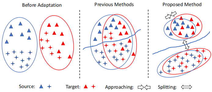
Left:在适应之前,源数据和目标数据之间存在域偏移;Middle:类不可知的自适应在域级将源数据和目标数据对齐,忽略了样本的类标签,因此可能导致次优解。因此,一个标签的目标样本可能与不同标签的源样本不一致;Right:我们的方法执行跨域的类感知对齐。为了避免错位,只减少了类内域的差异。将类间域差异最大化,提高了模型的泛化能力。
Middle 中的先前方法存在的问题:First, samples of different classes may be aligned incorrectly, e.g. both MMD and JMMD can be minimized even when the target-domain samples are misaligned with the source-domain samples of a different class. Second, the learned decision boundary may generalize poorly for the target domain.
本文提出的 CAN 网络(Contrastive Adaptation Network)优化了一个显式地对类内域差异和类间域差异建模的新度量,设计了一种交替更新 (alternating update)的训练策略,可以端到端(end-to-end)的方式进行。
2 Related Work
Class-agnostic domain alignment
MMD 距离(Maximum mean discrepancy),度量在再生希尔伯特空间中两个分布的距离,是一种核学习方法。 两个随机变量的距离为:
$\operatorname{MMD}[\mathcal{F}, p, q] := \underset{f \in \mathcal{F}}{\text{sup}} \left(\mathbf{E}_{p}[f(x)]-\mathbf{E}_{q}[f(y)]\right)$
$\operatorname{MMD}[\mathcal{F}, X, Y] :=\underset{f \in \mathcal{F}}{\text{sup}}\left(\frac{1}{m} \sum\limits _{i=1}^{m} f\left(x_{i}\right)-\frac{1}{n} \sum\limits_{i=1}^{n} f\left(y_{i}\right)\right)$
MMD距离的原始定义如上,$f$ 为属于函数域 $\mathcal{F}$ 中的函数,直观上理解就是两个分布经过一个定 义好的函数域 $\mathcal{F}$ 中的任意函数 $f$ 映射后的期望之差的最大值(上界)。在实际应用中,映射后的期望,通过样本均值来估计。一个直观的理解就是如果两个分布一样时,那么只要采样的样本足够多,那么不论函数域怎么定义,其 MMD 距离都是 $0$,因为不论通过什么样的函数映射后,两个一样的分布映射后的分布还是一样的,那么他们的期望之差都为 $0$ ,上界也就是 $0$。
$\operatorname{MMD}[\mathcal{F}, X, Y]=\left[\frac{1}{m^{2}} \sum\limits _{i, j=1}^{m} k\left(x_{i}, x_{j}\right)-\frac{2}{m n} \sum\limits_{i, j=1}^{m, n} k\left(x_{i}, y_{j}\right)+\frac{1}{n^{2}} \sum\limits_{i, j=1}^{n} k\left(y_{i}, y_{j}\right)\right]^{\frac{1}{2}}$
3 Problem Statement
Unsupervised Domain Adaptation (UDA) aims at improving the model's generalization performance on target domain by mitigating the domain shift in data distribution of the source and target domain. Formally, given a set of source domain samples $\mathcal{S}=\left\{\left(\boldsymbol{x}_{1}^{s}, y_{1}^{s}\right), \cdots,\left(\boldsymbol{x}_{N_{s}}^{s}, y_{N_{s}}^{s}\right)\right\}$ , and target domain samples $\mathcal{T}=\left\{\boldsymbol{x}_{1}^{t}, \cdots, \boldsymbol{x}_{N_{t}}^{t}\right\}$, $\boldsymbol{x}^{s}$ , $\boldsymbol{x}^{t}$ represent the input data, and $y^{s} \in\{0,1, \cdots, M-1\}$ denote the source data label of $M$ classes. The target data label $y^{t} \in\{0,1, \cdots, M-1\}$ is unknown. Thus, in UDA, we are interested in training a network using labeled source domain data $\mathcal{S}$ and unlabeled target domain data $\mathcal{T}$ to make accurate predictions $\left\{\hat{y}^{t}\right\}$ on $\mathcal{T}$ .
We discuss our method in the context ofdeep neural networks. In deep neural networks, a sample owns hierarchical features/representations denoted by the activations of each layer $l \in \mathcal{L}$ . In the following, we use $\phi_{l}(\boldsymbol{x})$ to denote the outputs of layer $l$ in a deep neural network $\Phi_{\theta}$ for the input $\boldsymbol{x}$ , where $\phi(\cdot)$ denotes the mapping defined by the deep neural network from the input to a specific layer.
4 Method
4.1 Maximum Mean Discrepancy Revisit
$\mathcal{D}_{\mathcal{H}}(P, Q) \triangleq \underset{f \sim \mathcal{H}}{\text{sup}} \left(\mathbb{E}_{\boldsymbol{X}^{s}}\left[f\left(\boldsymbol{X}^{s}\right)\right]-\mathbb{E}_{\boldsymbol{X}^{t}}\left[f\left(\boldsymbol{X}^{t}\right)\right]\right)_{\mathcal{H}} \quad\quad\quad(1)$
在实际应用中,对于第 $l$ 层,MMD 的平方值是用经验核均值嵌入来估计的:
$\begin{aligned}\hat{\mathcal{D}}_{l}^{m m d} & =\frac{1}{n_{s}^{2}} \sum_{i=1}^{n_{s}} \sum_{j=1}^{n_{s}} k_{l}\left(\phi_{l}\left(\boldsymbol{x}_{i}^{s}\right), \phi_{l}\left(\boldsymbol{x}_{j}^{s}\right)\right) \\& +\frac{1}{n_{t}^{2}} \sum_{i=1}^{n_{t}} \sum_{j=1}^{n_{t}} k_{l}\left(\phi_{l}\left(\boldsymbol{x}_{i}^{t}\right), \phi_{l}\left(\boldsymbol{x}_{j}^{t}\right)\right) \\& -\frac{2}{n_{s} n_{t}} \sum_{i=1}^{n_{s}} \sum_{j=1}^{n_{t}} k_{l}\left(\phi_{l}\left(\boldsymbol{x}_{i}^{s}\right), \phi_{l}\left(\boldsymbol{x}_{j}^{t}\right)\right)\end{aligned}\quad\quad\quad(2)$
其中,$x^{s} \in \mathcal{S}^{\prime} \subset \mathcal{S}$,$x^{t} \in \mathcal{T}^{\prime} \subset \mathcal{T}$,$n_{s}=\left|\mathcal{S}^{\prime}\right|$,$n_{t}=\left|\mathcal{T}^{\prime}\right|$。$\mathcal{S}^{\prime}$ 和 $\mathcal{T}^{\prime}$ 分别表示从 $S$ 和 $T$ 中采样的小批量源数据和目标数据。$k_{l}$ 表示深度神经网络第 $l$ 层选择的核。
4.2 Contrastive Domain Discrepancy
CDD 明确地考虑类信息,并衡量跨域的类内和类间的差异。最小化类内域差异以压缩类内样本的特征表示,而最大以类间域差异使彼此的表示更远离决策边界。联合优化了类内和类间的差异,以提高了自适应性能。所提出的对比域差异(CDD)是基于条件数据分布之间的差异。MMD 没有对数据分布的类型(例如边际或条件)的任何限制,MMD 可以方便地测量 $P\left(\phi\left(\boldsymbol{X}^{s}\right) \mid Y^{s}\right)$ 和 $Q\left(\phi\left(\boldsymbol{X}^{t}\right) \mid Y^{t}\right)$ 之间的差异:
$\mathcal{D}_{\mathcal{H}}(P, Q) \triangleq \sup _{f \sim \mathcal{H}}\left(\mathbb{E}_{\boldsymbol{X}^{s}}\left[f\left(\phi\left(\boldsymbol{X}^{s}\right) \mid Y^{s}\right)\right]-\mathbb{E}_{\boldsymbol{X}^{t}}\left[f\left(\phi\left(\boldsymbol{X}^{t}\right) \mid Y^{t}\right)\right]\right)_{\mathcal{H}}$
$\mu_{c c^{\prime}}\left(y, y^{\prime}\right)=\left\{\begin{array}{ll}1 & \text { if } y=c, y^{\prime}=c^{\prime} \\0 & \text { otherwise }\end{array}\right.$
其中,$c_1$ 和 $c_2$ 可以是不同的类,也可以是相同的类。
对于两类 $c_1$ 和 $c_2$,$\mathcal{D}_{\mathcal{H}}(P, Q)$ 平方的核平均嵌入估计为:
$ \hat{\mathcal{D}}^{c_{1} c_{2}}\left(\hat{y}_{1}^{t}, \hat{y}_{2}^{t}, \cdots, \hat{y}_{n_{t}}^{t}, \phi\right)=e_{1}+e_{2}-2 e_{3} \quad \quad\quad(3) $
Note:$\text{Eq.3}$ 定义了两种类感知域差异,1:当 $c_{1}=c_{2}=c$ 时,它测量类内域差异;2:当 $c_{1} \neq c_{2}$ 时,它成为类间域差异。
CDD 完整计算如下:
其中,$\hat{y}_{1}^{t}, \hat{y}_{2}^{t}, \cdots, \hat{y}_{n_{t}}^{t}$ 简写为 $\hat{y}_{1: n_{t}}^{t}$。
4.3 Contrastive Adaptation Network
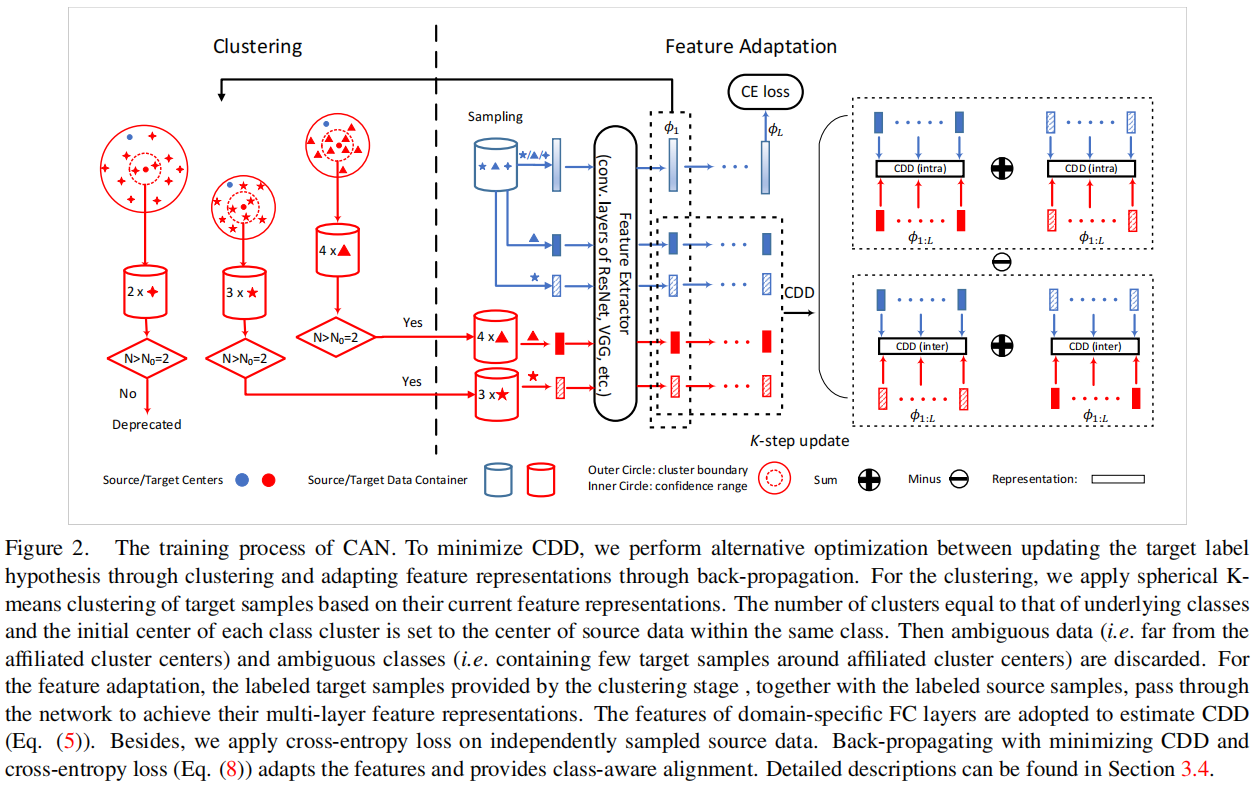
在本文中,我们从 ImageNet [7] 预训练网络开始,例如 ResNet [14,15],并将最后一个 FC 层替换为特定于任务的 FC 层。我们遵循一般的做法,将最后的 FC 层的域差异最小化,并通过反向传播来微调卷积层。然后,我们提出的 CDD 可以很容易地作为 FC 层激活的适应模块整合到目标中。我们将我们的网络命名为对比自适应网络(CAN)。总体目标:在深度 CNN 中,我们需要在多个 FC 层上最小化 CDD,即最小化
此外,通过最小化交叉熵损失来训练具有标签的源数据网络:
$\ell^{c e}=-\frac{1}{n^{\prime}} \sum\limits _{i^{\prime}=1}^{n_{s}^{\prime}} \log P_{\theta}\left(y_{i^{\prime}}^{s} \mid \boldsymbol{x}_{i^{\prime}}^{s}\right)\quad \quad\quad(7) $
其中,$y^{s} \in\{0,1, \cdots, M-1\}$ 代表源域中的样本 $\boldsymbol{x}^{s}$ 的标签,$P_{\theta}(y \mid \boldsymbol{x})$ 表示给定输入 $\boldsymbol{x}$,用 $\theta$ 参数化的标签 $y$ 的预测概率。
因此,总体目标可以表述为:
$\underset{\theta}{\text{min}}\quad \ell=\ell^{c e}+\beta \hat{\mathcal{D}}_{\mathcal{L}}^{c d d}\quad \quad\quad(8) $
请注意,我们对标记的源数据进行独立采样,以最小化交叉熵损失 $\ell^{c e}$,并估计 $\operatorname{CDD} \hat{\mathcal{D}}_{\mathcal{L}}^{c d d}$。通过这种方式,我们能够设计更有效的采样策略,以促进 CDD 的小批量随机优化,同时不干扰标记源数据的交叉熵损失的传统优化。
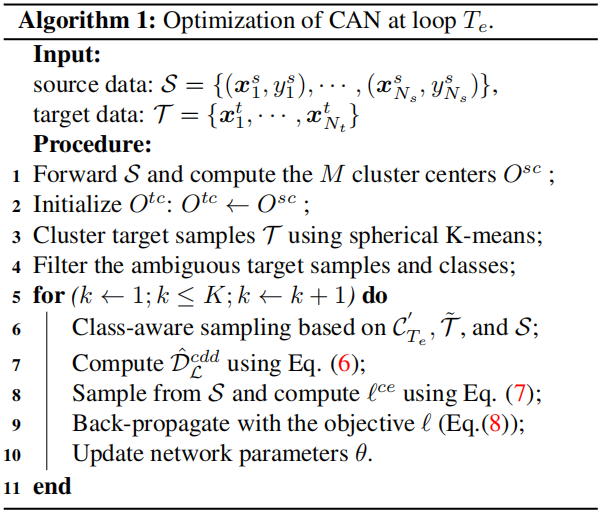
4.4 Optimizing CAN
CAN 的框架如 Figure2 所示。在本节中,我们主要集中讨论如何尽量减少 CAN 中的 CDD 损失。
4.4.1 Alternative optimization (AO)
如 $\text{Eq.5}$ 中所示,我们需要共同优化目标标签假设 $\hat{y}_{1: n_{t}}^{t}$ 和特征表示 $\phi_{1: L}$,本文采用了交替优化来执行这种优化。
假设有 $M$ 类,所以可以设置 $\mathrm{K}=\mathrm{M}$ 。
步骤:
1)使用源域的数据的表征计算每个类别的样本编码中心: $\mathrm{O}^{\mathrm{s}, \mathrm{c}}$ ,其中 $\mathrm{c}$ 是某个特定的类别,我们用这些源域中心初始化目标域的聚类的中心 $\mathrm{O}^{\mathrm{t}, \mathrm{c}}$ ,其中:
$\mathrm{O}^{\mathrm{sc}}=\sum_{i=1}^{\mathrm{n}_{\mathrm{s}}} 1_{y_{i}^{\mathrm{s}}=\mathrm{c}} \frac{\phi_{1}\left(\mathrm{x}_{\mathrm{i}}^{\mathrm{s}}\right)}{\left.\| \mathrm{x}_{\mathrm{i}}\right) \|}$$
$1_{y_{\mathrm{i}}^{\mathrm{s}}=\mathrm{c}}=\left\{\begin{array}{ll}1 & \text { if } \mathrm{y}_{\mathrm{i}}^{\mathrm{s}}=\mathrm{c} ; \\0 & \text { otherwise. }\end{array}, \mathrm{c}=\{0,1, \ldots, \mathrm{M}-1\}\right.$
2)计算样本与中心之间的距离,我们使用余弦距离,即:$\operatorname{dist}(\mathrm{a}, \mathrm{b})=\frac{1}{2}\left(1-\frac{\mathrm{a} \cdot \mathrm{b}}{\|\mathrm{a}\|\|\mathrm{b}\|}\right) $
3)聚类的过程是迭代的:
(1) 对每个目标域的样本找到所对应的聚类中心: $\hat{y}_{\mathrm{i}}^{\mathrm{t}}=\underset{c}{\arg \min \operatorname{dist}}\left(\phi\left(\mathrm{x}_{\mathrm{i}}^{\mathrm{t}}\right), \mathrm{O}^{\mathrm{tc}}\right) $;
(2) 更新聚类中心: $\mathrm{O}^{\mathrm{tc}} \leftarrow \sum_{\mathrm{i}=1}^{\mathrm{N}_{\mathrm{t}}} 1_{\hat{y}_{\mathrm{i}}^{\mathrm{t}}=\mathrm{c}}\frac{\phi_{1}\left(\mathrm{x}_{\mathrm{t}}^{\mathrm{t}}\right)}{\left\|\phi_{1}\left(\mathrm{x}_{\mathrm{i}}\right)\right\|}$
迭代直到收敛或者抵达最大聚类步数停止;
4)聚类结束后,每个目标域的样本 $\mathrm{x}_{\mathrm{i}}^{\mathrm{t}}$ 被赋予一个标签 $ \hat{y}_{\mathrm{i}}^{\mathrm{t}}$;
5)此外,设定一个阈值 $\mathrm{D}_{0} \in[0,1]$ ,将属于某个簇但是距离仍然超过给定阈值的数据样本删除,不参与本次计算 CDD,仅保留距离小于 $\mathrm{D}_{0}$ 的样本:
$\hat{\mathcal{T}}=\left(\mathrm{x}^{\mathrm{t}}, \hat{\mathrm{y}}^{\mathrm{t}}\right) \mid \operatorname{dist}\left(\phi_{1}\left(\mathrm{x}^{\mathrm{t}}\right), \mathrm{O}^{\mathrm{t}, \hat{\mathrm{y}}^{\mathrm{t}}}\right)<\mathrm{D}_{0}, \mathrm{x}^{\mathrm{t}} \in \mathcal{T}$
6)此外,为了提供更准确的样本分布的统计数据,假设每个类别挑选出来的集合 $ \hat{\mathcal{T}}$ 的大小至少包含某个数量 $N_{0}$ 的样本,不然这个类别本次也不参与计算 CDD,即最后参与计算的类别集为:
$\mathcal{C}_{T_{e}}=\left\{c \mid \sum_{i}^{|\mathcal{T}|} \mathbf{1}_{\hat{y}_{i}^{t}=c}>N_{0}, c \in \{0,1, \cdots, M-1\} \right \} $
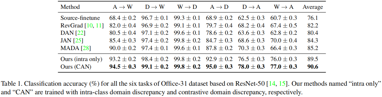
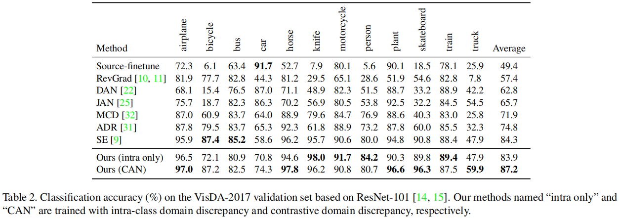
5 Experiment


评论区